Home

Lecture 13: Introduction to `JOIN`

Learning objective

Introduction to JOIN concepts
Table referencing and alias-ing
The INNER JOIN
Order of syntax and execution with JOIN queries

Warm up

Let’s pretend you have 2 small tables.

The employees table, which contains employees’ first and last names:

emp_no | first_name | last_name
-------+------------+-----------
 10001 | Georgi     | Facello   
 10002 | Bezalel    | Simmel    
 10003 | Parto      | Bamford   
 10004 | Chirstian  | Koblick   

The titles table, which contains employees’ job titles:

emp_no |      title      
-------+-----------------
 10004 | Senior Engineer
 10002 | Staff           
 10003 | Senior Engineer
 10001 | Senior Engineer

Manually, complete this table:

emp_no | first_name | last_name |   title
-------+------------+-----------|----------
 10001 | Georgi     | Facello   |
 10002 | Bezalel    | Simmel    |
 10003 | Parto      | Bamford   |
 10004 | Chirstian  | Koblick   |

What is a `JOIN`?

In the warm-up exercise above, what you did manually is the SQL equivalent of a JOIN between two tables.

A SQL JOIN connects data sources (tables) together in order to use information stored in multiple tables to display a desired result or output.

In the warm-up, we wanted to create an output that contains first_name and last_name (both stored in the employees table), as well as the employee title (which is stored in the title table). Thus, we need to connect the two data sources (employees table and title table) together, in order to display an unified output.

A simple example

To write the warm-up exercise in pseudo SQL:

SELECT *
FROM employees
JOIN titles
  ON employees.emp_no = titles.emp_no
;  

Let’s take this SQL apart, step by step, in the following section.

Key components of a `JOIN` SQL query

The tables

The first table named in a SQL query with JOIN is often referred to as the LEFT table, and the second table named is often referred to as the RIGHT table.

In this query:

SELECT *
FROM employees
JOIN titles
  ON employees.emp_no = titles.emp_no
;  

the LEFT table is: employees
the RIGHT table is titles

Hint: It might be easier to remember that the LEFT table is to the left of the JOIN SQL keyword, and that the RIGHT table is to the right of the JOIN SQL keyword, if the query is written in one single line, like so:

SELECT *
FROM employees JOIN titles ON employees.emp_no = titles.emp_no
;

However, for readability and styling purposes, the JOIN should be broken down into separate lines. Please see the SQL style guide for more details.

Exercise:

Which is the LEFT table and which is the RIGHT table, in the following JOIN query?

SELECT *
FROM titles
JOIN employees
  ON titles.emp_no = employees.emp_no
;  

The JOIN key columns

In the warm-up exercise, in order to make sure that the right job title is matched to the right employee first and last name, we use the emp_no column in both tables as the visual link connecting the correct employee names to their job titles.

For example, Georgi Facello has an emp_no of 10001, thus, their corresponding job title is Senior Engineer, which also has an emp_no of 10001.

In this SQL JOIN, emp_no is the common denominator field in both tables, thus, it is also known as the JOIN key column in both tables and serves as an unique identifier across the tables in the JOIN, making sure the right rows are joined together across the tables.

SELECT *
FROM employees
JOIN titles
  ON employees.emp_no = titles.emp_no
;  

the JOIN key column for employees is: the emp_no column in the employees table
the JOIN key column for titles is: the emp_no column in the titles table

Important Note

The key columns do not always share the same name, nor is it required for key columns to have the same names in order for the JOIN to succeed.

The requirements for the key columns are:

the JOIN key columns must be of the same data type (e.g. emp_no in both tables are both of the integer data type.) Otherwise, we will need to use CAST() to convert the data types.
the values inside columns are in common. (e.g. emp_no in both tables are used to store the employee ID numbers for those employed in this fictional company.)

Ordering matters (somewhat)

To use the two emp_no columns to link the two tables, the syntax requires a SQL reserve keyword ON, followed by setting the columns = to each other.

Unlike the tables, there is no LEFT or RIGHT positional reference for the JOIN key columns. In fact, the order of appearance of the column keys do not have any impact on the JOINs.

SELECT *
FROM employees
JOIN titles
  ON employees.emp_no = titles.emp_no
;  

can be re-written as the following, with no impact.

SELECT *
FROM employees
JOIN titles
  ON titles.emp_no = employees.emp_no
;  

For today’s lecture, the ordering of which table is the LEFT table and which table is the RIGHT table does not matter. However, once we start learning other types of JOINs (LEFT JOIN, RIGHT JOIN, etc.), the order of the tables in the JOIN will matter!

Explicit table references

The notation for employees.emp_no is an example of a <table_name>.<column_name> reference.

Previously, when we only had one table as data source, it was trivial to always indicate the table name.

We could have written:

SELECT
  first_name,
  last_name
FROM employees
;  

as:

SELECT
  employees.first_name,
  employees.last_name
FROM employees
;

but that seemed redundant and pointless.

However, with two tables as data sources, we need to always be explicit in naming which table the column(s) originate from.

Thus, in the JOIN ON clause, we specify the table names.

SELECT *
FROM employees
JOIN titles
  ON employees.emp_no = titles.emp_no
;  

This rule of referencing also applies in the SELECT clause and any other part of the SQL query statement.

If, instead of * as shorthand, we wish to call out each column separately, we can explicitly reference each column based on its source table.

Remember that in our warm-up abridged data tables:

employees table has the following columns: emp_no, first_name, last_name
titles table has the following columns: emp_no, title

Then, we can re-write our JOIN, instead of SELECT *, as:

SELECT
  employees.emp_no,
  employees.first_name,
  employees.last_name,
  titles.emp_no,
  titles.title
FROM employees
JOIN titles
  ON employees.emp_no = titles.emp_no
;  

Note that when using SELECT * with a 2 table JOIN, the LEFT table’s columns appear first, followed by the RIGHT table’s columns.

Table alias-ing

We’ve learned column alias-ing before:

SELECT
  original_column_name AS alias_column_name
FROM table
;

The convention for table alias-ing is to not use the keyword AS, but to rely on SQL to interpret the [space] between the original table name and the table alias name as an indication of alia-sing.

SELECT *
FROM original_table_name alias_table_name
;

Table alias-ing comes in handy now since we need to explicitly reference which column belongs to which table, which will generate a lot of repetition when writing a query.

For example, the original query:

SELECT
  employees.emp_no,
  employees.first_name,
  employees.last_name,
  titles.emp_no,
  titles.title
FROM employees
JOIN titles
  ON employees.emp_no = titles.emp_no
;  

after table aliasiing employees -> e and titles -> t, can be re-written, more concisely, as:

SELECT
  e.emp_no,
  e.first_name,
  e.last_name,
  t.emp_no,
  t.title
FROM employees e
JOIN titles t
  ON e.emp_no = t.emp_no
;  

Once established, the table alias can be referenced and used in any part of the same SQL query (e.g. in the SELECT, WHERE, GROUP BY, etc.)

Sidenote:

Alias-ing employees into a single letter e is not exactly best practice, though. Since, if the query gets long and complicated (100+ lines long), we might forget what e stands for.

Typically, table alias-ing is used to shorten a long multi-word table name into a single word. Given that our tables in the employees database tends to already be only one word, it’s also okay to forgo table alias-ing altogether, and continue to type out the full table name every time. The choice is up to you.

Breakout exercises

Ex 1. Using a variation of the pseudo tables in the warm-up exercise, note the column name changes.

The employees table, which contains employees’ first and last name:

emp_id | first_name | last_name
-------+------------+-----------
10001 | Georgi     | Facello   
10002 | Bezalel    | Simmel    
10003 | Parto      | Bamford   
10004 | Chirstian  | Koblick   

The titles table, which contains employees’ job titles:

emp_no |      title      
-------+-----------------
10001 | Senior Engineer
10002 | Staff           
10003 | Senior Engineer
10004 | Senior Engineer

Fill in the following pseudo code SQL to create a JOIN between the two tables:

SELECT *
FROM employees
JOIN titles
  ON ???.emp_id = ???.emp_no
;

Ex 2. Fill in the blank to construct a working SQL query using real tables in our PostgreSQL database. Feel free to run this against our PostgreSQL employees database for QA.

SELECT
  ???.first_name,
  ???.last_name,
  ???.birth_date,
  ???.from_date AS job_start_date,
  ???.to_date AS job_end_date
FROM employees
JOIN dept_emp
    ON employees.??? = dept_emp.???
LIMIT 10; -- for readability

Ex 3. Re-write the query from question 2. However, this time, alias the table dept_emp to department. Feel free to run this against our PostgreSQL employees database for QA.

The `INNER JOIN`

Being explicit about JOIN types

So far we have been writing:

SELECT *
FROM employees
JOIN titles
  ON employees.emp_no = titles.emp_no
;  

But, in reality, JOIN is just the default / shortened form of INNER JOIN:

SELECT *
FROM employees
INNER JOIN titles
  ON employees.emp_no = titles.emp_no
;  

There are many other types of JOINs (LEFT JOIN, RIGHT JOIN, FULL OUTER JOIN, CROSS JOIN, etc.), which we will cover in future lectures.

Just like how we should explicitly reference the table origin of a column, we should also be explicit about naming the type of JOIN being used in a query. Going forward, all JOINs will be fully written out as INNER JOINs.

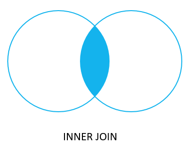
What is an INNER JOIN?

In a JOIN of two tables, an INNER JOIN only returns data if the value in the key column in the LEFT table also has a corresponding value in the key column in the RIGHT table.

The following Venn diagram illustrates how INNER JOIN clause works.

If in the employees table, the key column emp_no contains values (10001, 10002, 10003, 10004):

emp_no | first_name | last_name
-------+------------+-----------
 10001 | Georgi     | Facello   
 10002 | Bezalel    | Simmel    
 10003 | Parto      | Bamford   
 10004 | Chirstian  | Koblick   

and, if in the titles table, the key column emp_no also contains values (10001, 10002, 10003, 10004):

emp_no |      title      
-------+-----------------
10001 | Senior Engineer
10002 | Staff           
10003 | Senior Engineer
10004 | Senior Engineer

and, we apply the SQL:

SELECT *
FROM employees
INNER JOIN titles
  ON employees.emp_no = titles.emp_no
;  

then the output contains all 4 emp_no values as well:

emp_no | first_name | last_name |   title
-------+------------+-----------|----------------
 10001 | Georgi     | Facello   | Senior Engineer
 10002 | Bezalel    | Simmel    | Staff
 10003 | Parto      | Bamford   | Senior Engineer
 10004 | Chirstian  | Koblick   | Senior Engineer

However, if employees and titles contain different set of emp_no values:

employees table:

emp_no | first_name | last_name
-------+------------+-----------
 10001 | Georgi     | Facello   
 10002 | Bezalel    | Simmel    
 10003 | Parto      | Bamford   
 10004 | Chirstian  | Koblick   

titles table:

emp_no |      title      
-------+-----------------
10002 | Staff           
10003 | Senior Engineer
10004 | Senior Engineer
10005 | Senior Staff

and we apply the same SQL JOIN. Then, only the rows where the emp_no values are shared across both tables are returned:

emp_no | first_name | last_name |   title
-------+------------+-----------|----------------
 10002 | Bezalel    | Simmel    | Staff
 10003 | Parto      | Bamford   | Senior Engineer
 10004 | Chirstian  | Koblick   | Senior Engineer

Exercise

Given the following two tables, predict how many rows will be in the output of the JOIN query:

employees table:

emp_no | first_name | last_name
-------+------------+-----------
 10001 | Georgi     | Facello   
 10002 | Bezalel    | Simmel    
 10003 | Parto      | Bamford   

titles table:

emp_no |      title      
-------+-----------------
10004 | Senior Engineer
10005 | Senior Staff

SQL query:

SELECT *
FROM employees
INNER JOIN titles
  ON employees.emp_no = titles.emp_no
;  

Order of syntax and execution

Order of syntax

Previously, without JOINs, our order of syntax is as follows:

SELECT ...
FROM ... <data source>
WHERE ...
GROUP BY ...
HAVING ...
ORDER BY ...
LIMIT ...
;

Now, if the query includes a 2 table INNER JOIN, our new order of syntax is as follows:

SELECT ...
FROM ... <LEFT table>
INNER JOIN ... <RIGHT table>
  ON ...
WHERE ...
GROUP BY ...
HAVING ...
ORDER BY ...
LIMIT ...
;

Order of execution

Previously, all our data querying and manipulations are based off of the columns in a single table, where the table is referenced in the FROM clause of the SELECT statement.

However, the starting point for data source is no longer a single table, but the combination of all columns in the tables creating the JOIN.

Thus, our order of execution also needs to be adjusted:

PostgreSQL identifies the source table(s) using the FROM clause and any JOINs.
Filters rows based on WHERE filter conditions.
Aggregates and groups based on GROUP BY columns.
Additionally filters rows based on aggregated values using HAVING filter conditions.
Returns the columns specified (or temporarily created) using SELECT.
Sorts the order of rows using columns specified in ORDER BY.
Restricts number of rows outputted with LIMIT.

FROM and [JOIN] -> [WHERE] -> [GROUP BY] -> [HAVING] -> SELECT -> [ORDER BY] -> [LIMIT]

Let’s break down the following query step by step, according to the order of execution:

SELECT
  EXTRACT(year FROM dept_emp.from_date) AS start_year,
  COUNT(DISTINCT employees.emp_no) AS num_employees
FROM employees
INNER JOIN dept_emp
  ON employees.emp_no = dept_emp.emp_no
WHERE EXTRACT(year FROM employees.birth_date) BETWEEN 1950 AND 1960
GROUP BY 1
ORDER BY 1
LIMIT 3
;

PostgreSQL identifies the source table(s) using the FROM clause and any JOINs.

  SELECT *
  FROM employees
  INNER JOIN dept_emp
 ON employees.emp_no = dept_emp.emp_no
  ;

outputs:

  emp_no | birth_date |   first_name   |    last_name     | gender | hire_date  | emp_no | dept_no | from_date  |  to_date
  -------+------------+----------------+------------------+--------+------------+--------+---------+------------+------------
 10005 | 1955-01-21 | Kyoichi        | Maliniak         | M      | 1989-09-12 |  10005 | d003    | 1989-09-12 | 9999-01-01
 10010 | 1963-06-01 | Duangkaew      | Piveteau         | F      | 1989-08-24 |  10010 | d006    | 2000-06-26 | 9999-01-01
 10011 | 1953-11-07 | Mary           | Sluis            | F      | 1990-01-22 |  10011 | d009    | 1990-01-22 | 1996-11-09
 10013 | 1963-06-07 | Eberhardt      | Terkki           | M      | 1985-10-20 |  10013 | d003    | 1985-10-20 | 9999-01-01
  ... 331603 rows

Filters rows based on the WHERE filter conditions.

  SELECT *
  FROM employees
  INNER JOIN dept_emp
 ON employees.emp_no = dept_emp.emp_no
  WHERE EXTRACT(year FROM employees.birth_date) BETWEEN 1950 AND 1960
  ;

outputs:

  emp_no | birth_date |   first_name   |    last_name     | gender | hire_date  | emp_no | dept_no | from_date  |  to_date
  -------+------------+----------------+------------------+--------+------------+--------+---------+------------+------------
 10005 | 1955-01-21 | Kyoichi        | Maliniak         | M      | 1989-09-12 |  10005 | d003    | 1989-09-12 | 9999-01-01
 10010 | 1963-06-01 | Duangkaew      | Piveteau         | F      | 1989-08-24 |  10010 | d006    | 2000-06-26 | 9999-01-01
 10011 | 1953-11-07 | Mary           | Sluis            | F      | 1990-01-22 |  10011 | d009    | 1990-01-22 | 1996-11-09
 10013 | 1963-06-07 | Eberhardt      | Terkki           | M      | 1985-10-20 |  10013 | d003    | 1985-10-20 | 9999-01-01
  ... 227753 rows

Aggregates and groups based on GROUP BY columns.

  SELECT
 EXTRACT(year FROM dept_emp.from_date) AS start_year,
 COUNT(DISTINCT employees.emp_no) AS num_employees
  FROM employees
  INNER JOIN dept_emp
 ON employees.emp_no = dept_emp.emp_no
  WHERE EXTRACT(year FROM employees.birth_date) BETWEEN 1950 AND 1960
  GROUP BY 1
  ;

outputs:

  start_year | num_employees
 ------------+---------------
     1985 |         12475
     1986 |         13778
     1987 |         13900
     ...
     2002 |          1302
 (18 rows)        

Additionally filters rows based on aggregated values using HAVING filter conditions. There is no HAVING so this is passed.

Returns the columns specified (or temporarily created) using SELECT. This is done concurrently with step 3. So output is the same:

  start_year | num_employees
 ------------+---------------
     1985 |         12475
     1986 |         13778
     1987 |         13900
     ...
     2002 |          1302
 (18 rows)        

Sorts the order of rows using columns specified in ORDER BY.

Restricts number of rows outputted with LIMIT. Step 6 and step 7 combined gives us the top 3, as ranked by start year.

  start_year | num_employees
  -----------+---------------
     1985 |         12475
     1986 |         13778
     1987 |         13900
  (3 rows)

Breakout exercises

Ex 1. Re-order this SQL until it runs correctly:

GROUP BY 1, 2
ORDER BY 1, 2
INNER JOIN dept_emp d
FROM employees e
SELECT
  EXTRACT(year FROM d.from_date) AS hire_year,
  EXTRACT(month FROM d.from_date) AS hire_month,
  COUNT(
        DISTINCT
          CASE
            WHEN e.gender = 'F' THEN e.emp_no
          END
        ) AS num_female_employees_hired
ON e.emp_no = d.emp_no
;

Ex 2. Once the query in question 1 is running correctly, please label the order of execution for each part of the SQL query AND provide a layman’s term explanation of what the query is outputting.

Ex 3 (Challenge). Please create a multi-table INNER JOIN query between the dept_emp table, the employees table, and another table in the employees database so that the output has the following columns:

emp_no
first_name
last_name
dept_no
dept_name

Ex 4. Amend the SQL from question 3 so that the output is filtered and only displays employees that belong to the Development department.

Resources

Postgresql tutorial on table alias-ing.
Postgresql tutorial introduction to joins.
Postgresql tutorial on INNER JOIN.

Wrapping up

Reminder that both the in-class lab and homework 6 are due via Gradescope next Monday!

Home

Lecture 13: Introduction to JOIN

Learning objective

Warm up

What is a JOIN?

Key components of a JOIN SQL query

The INNER JOIN

Order of syntax and execution

Breakout exercises

Resources

Wrapping up

Lecture 13: Introduction to `JOIN`

What is a `JOIN`?

Key components of a `JOIN` SQL query

The `INNER JOIN`